Pycon 2016 tensorflow 研讨会总结 — tensorflow 手把手入门 #第二讲 word2vec

上一期我们讲到Pycon 2016 tensorflow 研讨会总结 — tensorflow 手把手入门 #第一讲 . 今天是我们第二讲, 来趴一趴word2vec.

什么是word2vec?

用来学习文字向量表达的模型 (相关文本文字的的特征向量).

• 向量空间模型解决了NLP中数据稀疏问题, 如果文字是离散的. 即, 把文字映射到相邻的空间点上.

立刻上图感受一下word2vec:

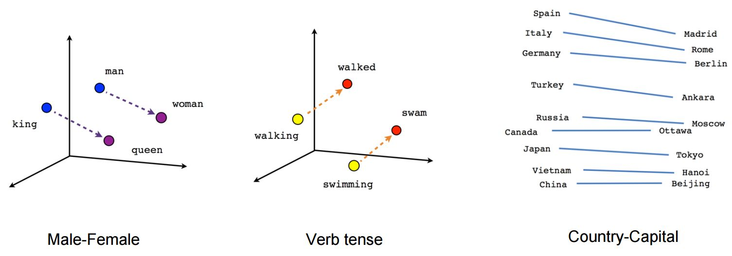
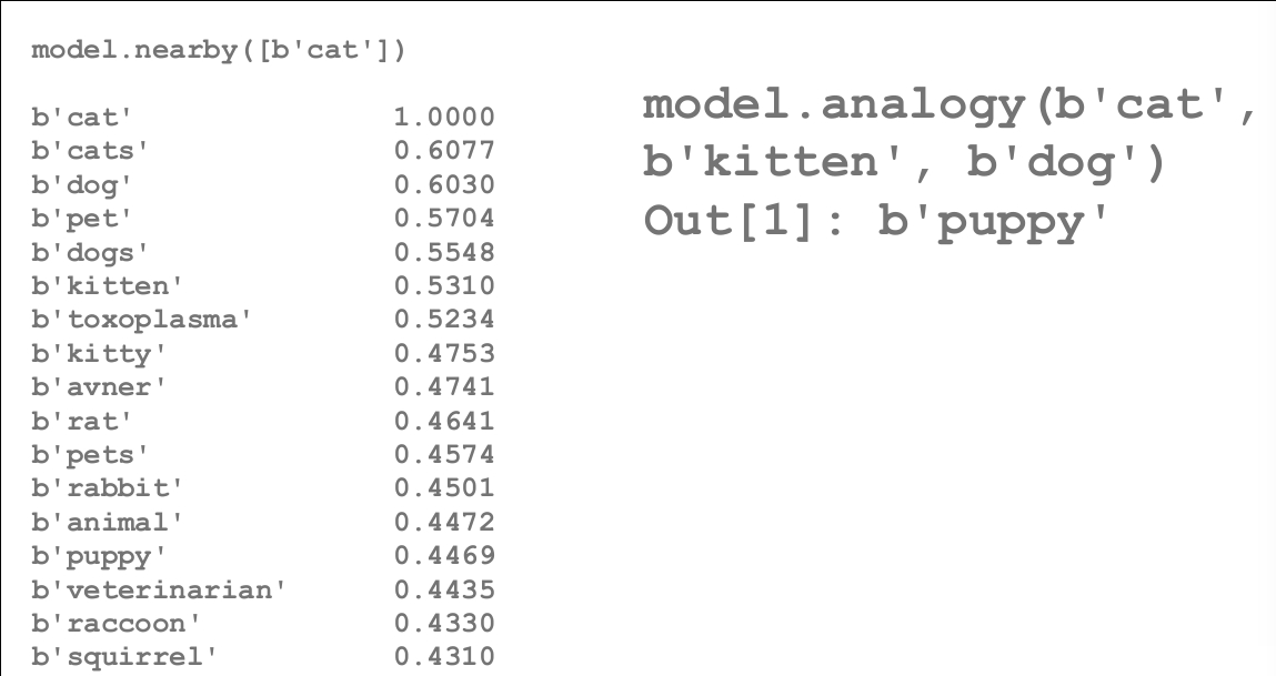
这里看看与文字’Cat’接近的词汇, 一目了然啊~如果一定要给’cat’一个向量描述, 上图左边这一列特征和权重是不是挺合理的呢? 嘿嘿~~~

word2vec两种方法:

• 基于计数的(如, LSA)
• 预测型的: 试着用学习到的embeddings在相邻文字中预测文字(如, word2vec 和 其他神经概率语言模型)

Mikolov等人的NIPS论文, http://bit.ly/word2vec-paper

两种word2vec

• 连续Bag-of-Words (COBW)
  • 从上下文来预测一个文字

• Skip-Gram
  • 从一个文字来预测上下文

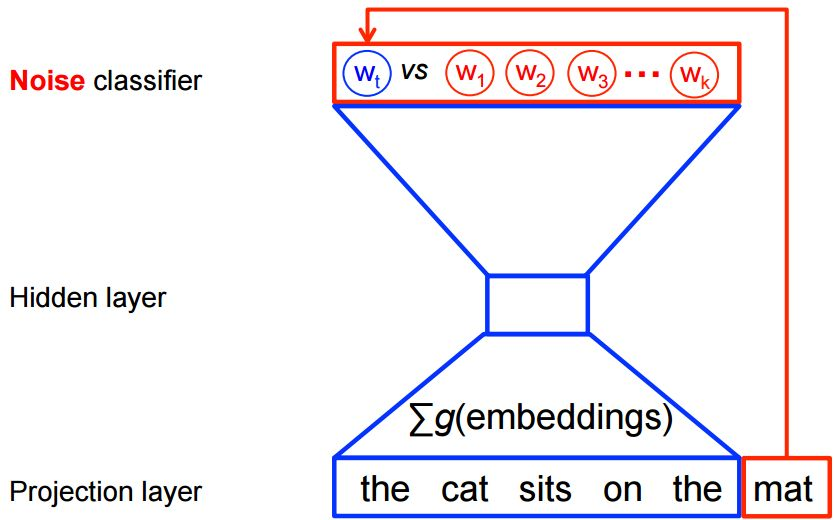
使得word2vec可扩展

• 使用对数回归把文字从假造的噪声文字中区分出来, 而不是使用完全的概率模型.
• 噪音对比估计(NCE) 损失.
  • tf.nn.nce_loss()
  • 用噪音文字扩展

Skip-Gram 模型(用目标文字预测上下文)

上下文/目标文字组合, 双向窗口大小为1:

the quick brown fox jumped over the lazy dog … →
([the, brown], quick), ([quick, fox], brown), ([brown,
jumped], fox),

输入/输出组合:

(quick, the), (quick, brown), (brown, quick), (brown,
fox), …

一般用SGD随机梯度下降优化

word2vec Tensorflow代码实例

# -*- coding: utf-8 -*-
# Copyright 2015 Google Inc. All Rights Reserved.
#
# Licensed under the Apache License, Version 2.0 (the "License");
# you may not use this file except in compliance with the License.
# You may obtain a copy of the License at
#
# http://www.apache.org/licenses/LICENSE-2.0
#
# Unless required by applicable law or agreed to in writing, software
# distributed under the License is distributed on an "AS IS" BASIS,
# WITHOUT WARRANTIES OR CONDITIONS OF ANY KIND, either express or implied.
# See the License for the specific language governing permissions and
# limitations under the License.
# ==============================================================================


# 导入一些库
import collections
import math
import os
import random
import time
import zipfile

import numpy as np
from six.moves import urllib
from six.moves import xrange # pylint: disable=redefined-builtin
import tensorflow as tf

# 第一步: 下载数据.
url = 'http://mattmahoney.net/dc/'


def maybe_download(filename, expected_bytes):
 """如果文件存在, 下载文件, 并且保证文件大小正确"""
 if not os.path.exists(filename):
 filename, _ = urllib.request.urlretrieve(url + filename, filename)
 statinfo = os.stat(filename)
 if statinfo.st_size == expected_bytes:
 print('Found and verified', filename)
 else:
 print(statinfo.st_size)
 raise Exception(
 'Failed to verify ' + filename + '. Can you get to it with a browser?')
 return filename

filename = maybe_download('text8.zip', 31344016)


# 把数据读入到一个列表中, 每个元素就是一个单词啦.
def read_data(filename):
 """解压出的文件获取第一个文件, 作为单词列表"""
 with zipfile.ZipFile(filename) as f:
 data = f.read(f.namelist()[0]).split()
 return data

#单词总数: 17005207
words = read_data(filename)
print('Data size', len(words))

# 第二步: 构造字典, 把非常稀少的单词替换为"UNK"(未知的单词标记).
vocabulary_size = 50000


def build_dataset(words):
 count = [['UNK', -1]]
 count.extend(collections.Counter(words).most_common(vocabulary_size - 1))
 dictionary = dict()
 for word, _ in count:
 dictionary[word] = len(dictionary)
 data = list()
 unk_count = 0
 for word in words:
 if word in dictionary:
 index = dictionary[word]
 else:
 index = 0 # dictionary['UNK']
 unk_count += 1
 data.append(index)
 count[0][1] = unk_count
 reverse_dictionary = dict(zip(dictionary.values(), dictionary.keys()))
 return data, count, dictionary, reverse_dictionary

# data 是一个list, 按照文章的单词顺序记录了每个单词在我们字典dictionary中的index, 即出现频率排名
# count 是所有单词的计数dict
# dictionary是每个单词的出现频率排名, key是单词, value是排名
# reverse_dictionary是dictionary的key-value颠倒, key是排名, value是单词
data, count, dictionary, reverse_dictionary = build_dataset(words)
del words # Hint to reduce memory.
print('Most common words (+UNK)', count[:5])
print('Sample data', data[:10], [reverse_dictionary[i] for i in data[:10]])

data_index = 0


# 第三步: 为skip-gram模型生成训练块的函数
def generate_batch(batch_size, num_skips, skip_window):
 global data_index
 assert batch_size % num_skips == 0
 assert num_skips <= 2 * skip_window
 batch = np.ndarray(shape=(batch_size), dtype=np.int32)
 labels = np.ndarray(shape=(batch_size, 1), dtype=np.int32)
 span = 2 * skip_window + 1
 buffer = collections.deque(maxlen=span)
 for _ in range(span):
 buffer.append(data[data_index])
 data_index = (data_index + 1) % len(data)
 for i in range(batch_size // num_skips):
 target = skip_window # 在buffer中心的目标label
 targets_to_avoid = [skip_window]
 for j in range(num_skips):
 while target in targets_to_avoid:
 target = random.randint(0, span - 1)
 targets_to_avoid.append(target)
 batch[i * num_skips + j] = buffer[skip_window]
 labels[i * num_skips + j, 0] = buffer[target]
 buffer.append(data[data_index])
 data_index = (data_index + 1) % len(data)
 return batch, labels

batch, labels = generate_batch(batch_size=8, num_skips=2, skip_window=1)
for i in range(8):
 print(batch[i], reverse_dictionary[batch[i]],
 '->', labels[i, 0], reverse_dictionary[labels[i, 0]])

# 第四步: 建立并训练skip-gram模型.

batch_size = 128
embedding_size = 128 # embedding向量的维数, 即隐层维数
skip_window = 1 # 向左和向右考虑的单词数, 即向左向右仅考虑一个单词.
num_skips = 2 # 可以重复使用输入去生成label的次数.

# 我们随机生成集合抽样邻近单词,
# 这里我们选那些出现频率比较高的单词
valid_size = 16 # 评估相似性的单词随机集合.
valid_window = 100 # 在分布首部选择样本.
valid_examples = np.random.choice(valid_window, valid_size, replace=False)
num_sampled = 64 #错分的样本

graph = tf.Graph()

with graph.as_default():

 # 输入数据
 train_inputs = tf.placeholder(tf.int32, shape=[batch_size])
 train_labels = tf.placeholder(tf.int32, shape=[batch_size, 1])
 valid_dataset = tf.constant(valid_examples, dtype=tf.int32)

 # 如果没有GPU,就用CPU的选项
 with tf.device('/cpu:0'):
 # 在输入数据中寻找隐含层.
 embeddings = tf.Variable(
 tf.random_uniform([vocabulary_size, embedding_size], -1.0, 1.0))
 embed = tf.nn.embedding_lookup(embeddings, train_inputs)

 # 为NCE 损失构造变量
 nce_weights = tf.Variable(
 tf.truncated_normal([vocabulary_size, embedding_size],
 stddev=1.0 / math.sqrt(embedding_size)))
 nce_biases = tf.Variable(tf.zeros([vocabulary_size]))

 # 为训练输入计算平均NCE损失
 # tf.nce计算损失时, 自动拿一个新的错分样本
 loss = tf.reduce_mean(
 tf.nn.nce_loss(nce_weights, nce_biases, embed, train_labels,
 num_sampled, vocabulary_size))

 # 学习率为1.0的SGD优化器
 optimizer = tf.train.GradientDescentOptimizer(1.0).minimize(loss)

 # 为每个输入样本和所有隐含层计算cos相似度.
 norm = tf.sqrt(tf.reduce_sum(tf.square(embeddings), 1, keep_dims=True))
 normalized_embeddings = embeddings / norm
 valid_embeddings = tf.nn.embedding_lookup(
 normalized_embeddings, valid_dataset)
 similarity = tf.matmul(
 valid_embeddings, normalized_embeddings, transpose_b=True)

 # Tensorboard作图用的Summarywriter
 loss_summary = tf.scalar_summary("loss", loss)
 train_summary_op = tf.merge_summary([loss_summary])

 # 增加变量初始化
 init = tf.initialize_all_variables()

# 第五步: 开始训练!.
num_steps = 100001

with tf.Session(graph=graph) as session:

 init.run()
 print("Initialized")

 # Directory in which to write summary information.
 # You can point TensorBoard to this directory via:
 # $ tensorboard --logdir=/tmp/word2vec_basic/summaries
 # Tensorflow assumes this directory already exists, so we need to create it.
 timestamp = str(int(time.time()))
 if not os.path.exists(os.path.join("/tmp/word2vec_basic",
 "summaries", timestamp)):
 os.makedirs(os.path.join("/tmp/word2vec_basic", "summaries", timestamp))
 # 创建SummaryWriter
 train_summary_writer = tf.train.SummaryWriter(
 os.path.join(
 "/tmp/word2vec_basic", "summaries", timestamp), session.graph)

 average_loss = 0
 for step in xrange(num_steps):
 batch_inputs, batch_labels = generate_batch(
 batch_size, num_skips, skip_window)
 feed_dict = {train_inputs: batch_inputs, train_labels: batch_labels}

 # We perform one update step by evaluating the optimizer op (including it
 # in the list of returned values for session.run()
 # Also evaluate the training summary op.
 _, loss_val, tsummary = session.run(
 [optimizer, loss, train_summary_op],
 feed_dict=feed_dict)
 average_loss += loss_val
 # Write the evaluated summary info to the SummaryWriter. This info will
 # then show up in the TensorBoard events.
 train_summary_writer.add_summary(tsummary, step)

 if step % 2000 == 0:
 if step > 0:
 average_loss /= 2000
 # 平均损失是以往2000个输入的损失估计.
 print("Average loss at step ", step, ": ", average_loss)
 average_loss = 0

 # 注意! 这很耗CPU(每经过500步就会慢下来大约20%)
 if step % 10000 == 0:
 sim = similarity.eval()
 for i in xrange(valid_size):
 valid_word = reverse_dictionary[valid_examples[i]]
 top_k = 8 # number of nearest neighbors
 nearest = (-sim[i, :]).argsort()[1:top_k + 1]
 log_str = "Nearest to %s:" % valid_word
 for k in xrange(top_k):
 close_word = reverse_dictionary[nearest[k]]
 log_str = "%s %s," % (log_str, close_word)
 print(log_str)
 final_embeddings = normalized_embeddings.eval()


# 第六步: 可视化embeddings.
def plot_with_labels(low_dim_embs, labels, filename='tsne.png'):
 assert low_dim_embs.shape[0] >= len(labels), "More labels than embeddings"
 plt.figure(figsize=(18, 18)) # in inches
 for i, label in enumerate(labels):
 x, y = low_dim_embs[i, :]
 plt.scatter(x, y)
 plt.annotate(label,
 xy=(x, y),
 xytext=(5, 2),
 textcoords='offset points',
 ha='right',
 va='bottom')

 plt.savefig(filename)

try:
 from sklearn.manifold import TSNE
 import matplotlib.pyplot as plt

 tsne = TSNE(perplexity=30, n_components=2, init='pca', n_iter=5000)
 plot_only = 500
 low_dim_embs = tsne.fit_transform(final_embeddings[:plot_only, :])
 labels = [reverse_dictionary[i] for i in xrange(plot_only)]
 plot_with_labels(low_dim_embs, labels)

except ImportError:
 print("Please install sklearn and matplotlib to visualize embeddings.")

 

 

参考文献

重要的Tensorflow资料：

1. Tensorflow backgroud 是一个官方的Tensorflow动画教程非常棒：http://playground.tensorflow.org/
2. TFLearn：一个深度学习的tensorflow上层API库。https://github.com/tflearn/tflearn
3. 一些Tensorflow模型的实现： https://github.com/tensorflow/models

研讨会视频:

https://www.youtube.com/watch?v=GZBIPwdGtkk

研讨会PPT下载：