Brief History of Machine Learning 机器学习简史

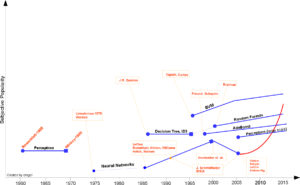
My subjective ML timeline

Since the initial standpoint of science, technology and AI, scientists following Blaise Pascal and Von Leibniz ponder about a machine that is intellectually capable as much as humans. Famous writers like Jules

Pascal’s machine performing subtraction and summation – 1642

Machine Learning is one of the important lanes of AI which is very spicy hot subject in the research or industry. Companies, universities devote many resources to advance their knowledge. Recent advances in the field propel very solid results for different tasks, comparable to human performance (98.98% at Traffic Signs – higher than human-).

Here I would like to share a crude timeline of Machine Learning and sign some of the milestones by no means complete. In addition, you should add “up to my knowledge” to beginning of any argument in the text.

First step toward prevalent ML was proposed by Hebb , in 1949, based on a neuropsychological learning formulation. It is called Hebbian Learning theory. With a simple explanation, it pursues correlations between nodes of a Recurrent Neural Network (RNN). It memorizes any commonalities on the network and serves like a memory later. Formally, the argument states that;

Let us assume that the persistence or repetition of a reverberatory activity (or “trace”) tends to induce lasting cellular changes that add to its stability.… When an  axon  of cell  A is near enough to excite a cell  B and repeatedly or persistently takes part in firing it, some growth process or metabolic change takes place in one or both cells such that  A’s efficiency, as one of the cells firing  B, is increased.[1]
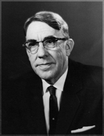
Arthur Samuel
Arthur Samuel

In 1952 , Arthur Samuel at IBM, developed a program playing Checkers . The program was able to observe positions and learn a implicit model that gives better moves for the latter cases. Samuel played so many games with the program and observed that the program was able to play better in the course of time.
继续阅读Brief History of Machine Learning 机器学习简史
[转] Ubuntu14.04LTS安装TensorFlow

1. Pip

如果已经安装过pip,可以跳过这里的安装步骤。

$ sudo apt-get install python-pip python-dev python-setuptools build-essential
$ sudo pip install --upgrade pip
$ sudo pip install --upgrade virtualenv

为了检测是否安装好,可以查看pip的版本:

$ pip --version
pip 8.1.2 from /usr/local/lib/python2.7/dist-packages (python 2.7)

2. Tensorflow

接下来,就可以按照Tensorflow Download and Setup中的Pip Installation开始安装,命令如下:

# Ubuntu/Linux 64-bit, CPU only:
$ sudo pip install --upgrade https://storage.googleapis.com/tensorflow/linux/cpu/tensorflow-0.8.0-cp27-none-linux_x86_64.whl
继续阅读[转] Ubuntu14.04LTS安装TensorFlow

#2 大话机器学习中的贝叶斯 Bayesian

#2 大话机器学习中的贝叶斯 Bayesian
/

这一期, 我们来谈一谈机器学习中的贝叶斯. 概率论中贝叶斯理论, 作为概率的一种“思考方式”, 十分通用. 当机器学习应用中, 贝叶斯的强大理论提现在多个领域, 包括超参数贝叶斯, 贝叶斯推断, 非参贝叶斯等等…

入门

机器学习中的贝叶斯, 首先要区分概率中频率学派和贝叶斯学派的. 网上有各种各样的解释, 其实, 我们可以从机器学习的角度去解释.

机器学习问题可以总结为: 找到一个好的 \theta 代表一个模型, \theta 表示这个模型的所有参数, 而这个模型就是我们能够训练出的最好模型(至少我们认为是最好的).  什么是最好的模型? 假设有未知数据集 X_{unknown} , 如果 P\left(X_{unknown}\middle|\theta\right) = 1 , 那么这个模型就是最好的. 当然这是不可能的, 也许只有上帝才能对所有的未知100%准确预测. 但我们一定是希望 P\left(X_{unknown}\middle|\theta\right) 越大越好, 趋向于1.

如何做到使得 P\left(X_{unknown}\middle|\theta\right) 越大越好 ? 这就引出了概率论中的两大学派: 传说中的”频率学派”和”贝叶斯学派”. 两大学派区别在哪里? 看下面这个公式:

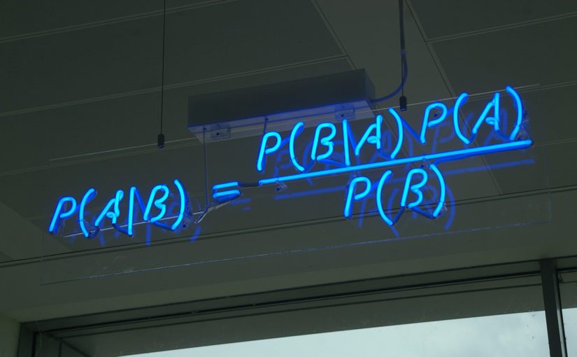
P\left(\theta\middle|X_{train}\right) = \frac{P\left(X_{train}\middle|\theta\right)P\left( \theta\right)}{P\left(X_{train}\right)}

没错! 这就是大名鼎鼎的贝叶斯公式 ! 机器学习中,  X_{train} 是真实的训练数据或者抽样数据 . P\left(\theta\middle|X_{train}\right) 是后验概率(posterior)分布 . P\left(X_{train}\middle|\theta\right)是似然概率(likelihood).   P\left( \theta\right) 是先验概率分布(prior). P\left(X_{train}\right)是归一化”证据”(evidence)因子.

“频率学派”认为, 后验概率和先验概率都是不存在的, 模型 \theta 不论简单复杂, 参数已经是上帝固定好了的, 只要根据大数定理, 当训练数据足够大, 我们就能找到那个最好的 \theta . 于是公式变为:

 P\left(X_{train}\right) = P\left(X_{train}\middle|\theta\right)

无论有没有 \theta , 抽样数据 X_{train} 出现的概率都是一样的, 因为任何数据都是从上帝指定的模型中生成的. 于是我们找到 \theta 的任务就很简单, 最大化 P\left(X_{train}\middle|\theta\right) 似然概率就行了. 数据量越大, 模型拟合度越高, 我们越相信得到的 \theta 越接近上帝指定的那个 \theta. 所以”频率学派”预测投硬币正反的概率的方法就是, 投10000次硬币吧, 看看正面出现多少次. 这种基于统计的预测有很多缺点, 首先它指定了一个固定概率, 如果上帝指定的模型不是固定的呢? 另外, 如果数据量不足够大, 预测会不会非常不准确? 当数据维数增大时, 实际计算量也会变得非常大.

“贝叶斯学派”认为, 人类的知识是有限的, 我们不知道上帝的安排, 就先假设一个先验(我们已有的知识), 再根据训练数据或抽样数据, 去找到后验分布, 就能知道模型最可能是个什么样子. 继续阅读#2 大话机器学习中的贝叶斯 Bayesian